Primal-Dual Mumford-Shah
1. Mumford-Shah Functional
Firstly, we introduce the Mumford-Shah Functional from paper Optimal approximations by piecewise smooth functions and associated variational problems
We have the g the “image” data, whose domain is in \(R\subset \mathbb{R}^{2}\), and f : \(\cup R_{i \to \mathbb{R}}\) a differentiable smooth function on \(\cup R_{i}\)
Here we consider to segment the image into \(\{ R_{i}\}\), disjoint connected open subsets of R. \(\Gamma\) will be the union of the part of the boundary of \(R_{i}\) inside R, so that :
And the Mumford-Shah Function is defined as a energy function:
Where we have the first term: to ensure f is close to g. The second term: that f is smooth within the region \(R_{i}\). And the third term , to achieve short boundaries. All the three terms are important, without anyone of them, we will always have a zero optimal trival solution.
1.1 Piecewise constant
The paper discussed several special cases of the functional. Firstly \(E_{0}\), which restrict f to be a piecewise constant function. Alors, the gradient terms of the energy function will be zero. And f(x) in each area will be the mean of g : \(mean_{R_{i}}(g)\) , we define :
If \(\Gamma\) fixed , and \(\mu\to 0\), f minimize E tends to be a such piecewise constant . That we have : \(E_{0}\) is the natural limit functional of E as \(\mu \to 0\).
In this case, it will be a The Plateau problem .
1.2 \(E_{\infty}\)
The authors also descussed \(E_{\infty}\) :
Generalized deodesic problem :
- \(E_{\infty}\) tends to make length of \(\Gamma\) as short as possible.
- \(E_{\infty}\) tends to make g has the largest possible derivative when normal to \(\Gamma\).
If we define the solution f to be g when far from the boundaries and take \(f_{\infty}\) when very close to \(\Gamma\) :
Where \(\mu = 1/\epsilon, \ \nu = \epsilon \nu_{infty}\), With this f function, we will have :
While \(\mu \to \infty\) we will have \(\epsilon \to 0\). That we have : \(E_{\infty}\) is the natural limit functional of E as \(\mu \to \infty\).
2. Convex Relaxation
This convex relaxation is introduced by An algorithm for minimizing the mumford-shah functional Which is also the basic for chapter 3, in this page.
The notaion of Mumford-Shah functional in this article:
Where we have f the known observation of the image, \(f:\Omega\subset \mathbb{R}^{2} \to \mathbb{R}\), and \(u:\Omega\to\mathbb{R}\) a piece wise smooth function (our desired solution).
I skip the related works here, as I haven’t read them (paper worth reading An efficient primal-dual hybrid gradient algorithm for total variation image restoration ).
2.1 Step 1
Step 1 : this article try to reform the formule of Mumford-Shah functional, by defining \(u\in SBV(\Omega)\) , the special functions of bounded variation [1] . And define the upper level sets of u by the characteristic function \(\mathbf{1}_{u} : \Omega \times \mathbb{R}\to \{0,1\}\) of the subgraph of u :
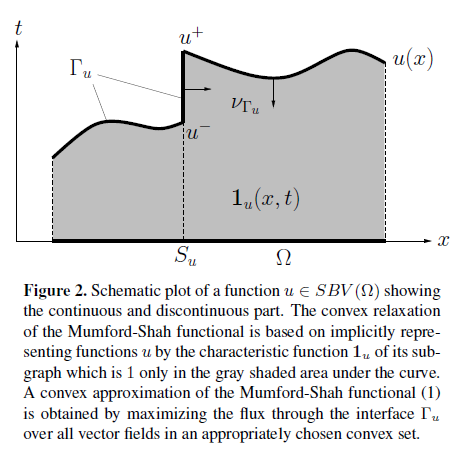
| [1] | i.e. functions u of bounded variation for which the derivative Du is the sum of an absolutely continuous part \(\triangledown u \cdot dx\) and a discontinuous singular part \(S_{u}\), see Figure 2. |
2.2 Step 2
Step 2 : Theorem 1. For a function \(u\in SBV(\Omega)\) the Mumford-Shah functional can be written as :
with a convex set :
Proof Theorem 1. : First we observe that the right hand part, the intergration, is a integration of changement of the space \(\Omega\times \mathbb{R}\), It is equivalent to the intergraion of the energy flow on the boundary (the normal of the function at boundaries \(\nu_{\Gamma_{u}}\)):
As in the boundary \(\Omega\setminus S_{u}\), we have the gradient w.r.t. t zero, and w.r.t. x \(\triangledown u\), followed by a normalization step. And in \(S_{u}\), we have the gradient w.r.t. t zero, and w.r.t. x the unit vector pointing from outside to inside. Taking this expression into the integration :
If we add constraints that :
Which is the constraint that \(\varphi\) lies in the convex set K. And it imples that :
We could further prove that this difference is rather small, that we could assume it is an equal, with an arbitrarily small error. \(\square\) .
2.3 Step 3
Step 3. Relaxation in the upper reformed Mumford-Shah function, the characteristic function \(\mathbf{1}_{u}\) is a non-convex function. Here we apply a convex relaxation upon this part. Introduce a generic function \(v(x,t):\Omega\times\mathbb{R}\to [0,1]\) to substitue \(\mathbf{1}_{u}\) , which satisfies:
Finally, we obtain the relaxed convex optimization problem :
2.4 Discrete Setting
Consider the discrete case. Use a regular \((N\times N)\times M\) pixel gird in space \(\Omega \times \mathcal{R}\) :
- Authors define the discrete space C for v :
- And develop a discrete version of convex set K.
- The discrete graident operator could be expressed by a matrix A.
Then we have a discrete version of the problem:
2.5 Primal-Dual method
Here the authors consider a more general problem:
Which is a seddle-point problem, and will be solved by sequential apply Newton’s method to the two variables. The convergence proof could be seen in the paper.
Where \(\tau\) and \(\sigma\) are choosen based on \(\tau\sigma L^{2}<1\) (L : the Lipschitz parameter). And the projection onto K is calculated using Dykstra’s iterative projection algorithm [2] (A method for finding projections onto the intersection of convex sets in Hilbert spaces ).
| [2] | In the next paper, these projections will be generalized to solve using the properties of Moreau’s theorem, and the resolvent operator. Or we could intreprete it as the proximal algorithm . |
3. First-order Primal-Dual
3.1 Primal-Dual formulation
From the paper A first-order primal-dual algorithm for convex problems with applications to imaging . Here a more general saddle-point problem is considered:
where \(G: X\to [0, +\infty]\) and \(F^{*} : Y\to [0,+\infty]\) are proper, convex, lower-semicontinous (l.s.c) functions. \(F^{*}\) being itself the convex conjugate of a convex l.s.c. function F.
This saddle-point problem is a primal-dual formulation of the nonlinear primal problem :
or of the corresponding dual problem:
The nonlinear primal problem is equivalent to the problem :
The lagrangian function is :
We have the dual function :
The beginning of this article shows various of the properties of the resolvent, which has close relation with the proximal operator .
Especially, that the resolvent operator and the proximal operator are equivalent interpretation .
And the Moreau’s decomposition theorem .
3.2 Algorithm
- Initialization : Choose \(\tau, \sigma >0, \theta\in [0,1]\), \((x^{0}, y^{0}) \in X\times Y\), and set \(\bar{x}^{0} = x^{0}\).
- Iterations : Update \(x^{n}, y^{n}, \bar{x}^{n}\) as follows:
Taking \(\theta\) equals 0, will result in the classical Arrow-Hurwicz algorithm. And this paper takes \(\theta\) to be 1. which can be seen as an approximate extragradient step.
