2. Properties

2.1 Separable sum

If f is seperable across two variables, so \(f(x,y) = \phi(x) + \psi(y)\), then:

\[\mathbf{prox}_{\lambda f}(v, w) = (\mathbf{prox}_{\lambda \phi}(v), \mathbf{prox}_{\lambda \psi}(w))\]

Proof:

\[\begin{split}\begin{align*} \mathbf{prox}_{\lambda f}(v, w) & = \mathop{\arg\min}_{x, y} (f(x, y) + \frac{1}{2 \lambda}\| \begin{bmatrix} x \\ y \end{bmatrix} - \begin{bmatrix} v \\ w \end{bmatrix} \|_{2}^{2}) \\ &= \mathop{\arg\min}_{x, y} (\phi(x) + \psi(y) + \frac{1}{2 \lambda}\| x - v\|_{2}^{2} + \frac{1}{2 \lambda}\| y - w \|_{2}^{2}) \\ &= (\mathbf{prox}_{\lambda \phi}(v), \mathbf{prox}_{\lambda \psi}(w)) \end{align*}\end{split}\]

2.2 Basic operations

2.2.1 Post-Composition

If \(f(x) = \alpha \phi(x) + b\), with \(\alpha > 0\), then:

\[\mathbf{prox}_{\lambda f}(v) = \mathbf{prox}_{\alpha \lambda \phi}(v)\]

Proof:

\[\begin{split}\begin{align*} \mathbf{prox}_{\lambda f}(v) & = \mathop{\arg\min}_{x} (\alpha\phi(x) + b + \frac{1}{2 \lambda}\| x - v\|_{2}^{2}) \\ &= \mathop{\arg\min}_{x} \alpha(\phi(x) + \frac{1}{2 \lambda \alpha}\| x - v\|_{2}^{2}) \\ &= \mathbf{prox}_{\alpha \lambda \phi}(v) \end{align*}\end{split}\]

2.2.2 Pre-Composition

If \(f(x) = \phi(\alpha x + b)\), with \(\alpha \ne 0\), then:

\[\mathbf{prox}_{\lambda f}(v) = \frac{1}{\alpha}(\mathbf{prox}_{\alpha^{2} \lambda \phi}(\alpha v +b) - b)\]

Proof:

\[\begin{split}\begin{align*} \mathbf{prox}_{\lambda f}(v) & = \mathop{\arg\min}_{x} (phi(\alpha x+b) + \frac{1}{2 \lambda}\| x - v\|_{2}^{2}) \\ &= \mathop{\arg\min}_{x} \alpha(\phi(\alpha x+b) + \frac{1}{2 \lambda \alpha^{2}}\| (\alpha x +b) - (\alpha v +b)\|_{2}^{2}) \\ &= \frac{1}{\alpha}(\mathbf{prox}_{\alpha^{2} \lambda \phi}(\alpha v +b) - b) \end{align*}\end{split}\]

If \(f(x) = \phi(Q x )\), with Q orthogonal, then:

\[\mathbf{prox}_{\lambda f}(v) = Q^{T}\mathbf{prox}_{\lambda \phi}(Q v )\]

2.2.3 Affine addition

If \(f(x) = \phi(x) + a^{T}x + b\), then :

\[\mathbf{prox}_{\lambda f}(v) = \mathbf{prox}_{\lambda \phi}(v - \lambda a)\]

Proof:

\[\begin{split}\begin{align*} \mathbf{prox}_{\lambda f}(v) &= \mathop{\arg\min}_{x} (phi(x) + a^{T}x + b + \frac{1}{2 \lambda}\| x - v\|_{2}^{2}) \\ &= \mathop{\arg\min}_{x} (phi(x) + \frac{1}{2 \lambda}(x^{T}x + v^{T}v - 2v^{T}x + 2 \lambda a^{T}x) ) \\ &= \mathop{\arg\min}_{x} (phi(x) + \frac{1}{2 \lambda}(x^{T}x + v^{T}v - 2(v^{T} - \lambda a^{T})x)) ) \\ &= \mathbf{prox}_{\lambda \phi}(v - \lambda a) \end{align*}\end{split}\]

In the last few equations, notices that we can add term of a and v.

2.2.4 Regularization

If \(f(x)=\phi(x) + (\frac{\rho}{2} \| x- a\|^{2}_{2})\), then:

\[\mathbf{prox}_{\lambda f}(v) = \mathbf{prox}_{\bar{\lambda} \phi}(\frac{\bar{\lambda}}{\lambda}v - (\rho \bar{\lambda})a)\]

where \(\bar{\lambda} = \lambda /(1+\lambda \rho)\)

2.2.5 Fixed Points

The point \(x^{*}\) minimizes f if and only if:

\[x^{*} = \mathbf{prox}_{\lambda f}(x^{*})\]

Proof: Can be found in the paper chapter 2.

2.2.6 Lipschitz continuous

(Mostly from Wikipedia) Given two metric space \((X, d_{X})\) and \((Y, d_{Y})\), where \(d_{X}\) denotes the metric on the set X and \(d_{Y}\) is the metric on the set Y, a function \(f : X \to Y\) is called Lipschitz continuous, if exist a constant \(K \in \mathbf{R}; K > 0\), such that for any \(x_{1}, x_{2} \in X\) :

\[d_{Y}(f(x_{1}), f(x_{2})) \le K d_{X}(x_{1}, x_{2})\]

For an example, if we have \(f : \mathbf{R} \to \mathbf{R}\), and in a l2 space then :

\[\| f(x_{1}), f(x_{2}) \|_{2} \le K \| x_{1}, x_{2} \|_{2}\]

We can easily see that, if \(K \le 1\), then the distance of function value space be smaller than then the distance in original space.

2.2.7 Fixed point algorithms

We can use the properties above to find a converging sequence to get closer to the optimal position, which is the fixed point. We have, if the Lipschitz continuous with constant K less than 1 (non-expansiveness), then we can repeatedly applying \(\mathbf{prox}_{f}\) to converge to the fixed point. As we have :

\[\| \mathbf{prox}_{f}(x) - \mathbf{prox}_{f}(y) \|_{2}^{2} \le (x-y)^{T}(\mathbf{prox}_{f}(x) - \mathbf{prox}_{f}(y))\]

The simplest proximal method should be :

\[x^{k+1} = \mathbf{prox}_{\lambda f}(x^{k})\]

2.3 Proximal average

Let \(f_{1}, ..., f_{m}\) be closed proper convex functions, Then we have that :

\[\frac{1}{m} \sum_{i=1}^{m} \mathbf{prox}_{f_{i}} = \mathbf{prox}_{g}\]

Where g could be called the proximal average of \(f_{1}, ..., f_{m}\).

2.4 Moreau decomposition

This is an important property. It is closly connected to the duality, and the Moreau envelope. The main materials for this part from the paper, Wiki for cvx and Math 301.

2.4.1 Projection mapping

Define the projection mapping of a hilbert space.

Let \((\mathbb{H},\langle\cdot,\cdot\rangle)\) be a Hilbert space and \(\mathbf{C}\) a closed convex set in \(\mathbb{H}\), tge projection mapping \(P_{\mathbb{C}}\) onto \(\mathbb{C}\) is the mapping \(P_{\mathbb{C}} : \mathbb{H} \to \mathbb{H}\), defined by \(P_{\mathbb{C}} \in \mathbf{C}\) and :

\[\| x - P_{\mathbf{c}}(x) \| = \min (\| x - y \|; y \in \mathbf{C})\]

2.4.2 Characterization

Let \((\mathbb{H},\langle\cdot,\cdot\rangle)\) be a Hilbert space, \(\mathcal{C}\) a closed convex set in \(\mathbb{H},\,u\in\mathbb{H}\)

and \(v\in\mathcal{C}\). Then \(v=P_{\mathcal{C}}(u)\) if and only if \(\langle u-v,w-v\rangle\leq0\) for all \(w\in\mathcal{C}\).

Proof: can be seen Wiki for cvx.

2.4.3 Moreau’s theorem

Moreau’s theorem is a fundamental result characterizing projections onto closed convex cones in Hilbert spaces.

Recall that a convex cone in a vector space is a set which is invariant under the addition of vectors and multiplication of vectors by positive scalars.

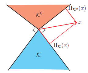
Theorem (Moreau): Let \(\mathcal{K}\) be a closed convex cone in the Hilbert space \((\mathbb{H},\langle\cdot,\cdot\rangle)\)

and \(\mathcal{K}^\circ\) its polar cone; that is, the closed convex cone defined by \(\mathcal{K}^\circ=\{a\in\mathbb{H}\,\mid\,\langle a,b\rangle\leq0,\,\forall b\in\mathcal{K}\}\).

For \(x,y,z\in\mathbb{H}\) the following statements are equivalent:

1. \(z=x+y,\,x\in\mathcal{K},\,y\in\mathcal{K}^\circ\) and \(\langle x,y\rangle=0\);
2. \(x=P_{\mathcal{K}}z\) and \(y=P_{\mathcal{K}^\circ}z\).

Attention that \(\mathcal{K}^\cdot\) its dual cone is defined as \(\mathcal{K}^\cdot=\{a\in\mathbb{H}\,\mid\,\langle a,b\rangle\ge0,\,\forall b\in\mathcal{K}\}\). The following image is in a Euclidean space, the Moreau’s theorem can be seen as an decomposition by the projection in the two convex cone (that is dual of each other).

Proof: can be seen Wiki for cvx.

2.4.4 Moreau decomposition

The following relation always holds :

\[v = \mathbf{prox}_{f}(v) + \mathbf{prox}_{f^{*}}(v)\]

where :

\[f^{*}(y) = \sup_{x} (y^{T}x - f(x))\]

is the convex conjugate of f.

2.4.5 Proof 1. Moreau decomposition

1. Re-note \(x=\mathbf{prox}_{f}(v)\), and \(y = v - x\). So it remains to prove \(y=\mathbf{prox}_{f^{*}}(v)\)
2. From the difinition:

\[x = \mathbf{prox}_{f}(v) = \mathop{\arg\min}_{x} (f(x) + \frac{1}{2}\| x - v \|_{2}^{2})\]

Using the optimal condition, we have:

\[0 \in \partial(f(x) + \frac{1}{2}\| x - v \|_{2}^{2}) = \partial f(x) + (x-v)\]

Where \(\partial f\) is the subgradient set of f. So we have \(v - x \in \partial f(x)\), then \(y \in \partial f(x)\).

3. To prove \(y = \mathbf{prox}_{f^{*}}(v)\). As \(y \in \partial f(x)\), it is equivalent to \(0 \in y - \partial f(x)\), so \(0 \in \partial_{x} (y^{T}x - f(x))\), it means, there exists some affine minorat of f with slope y which is exact at x.

\[f^{*}(y) = y^{T}x - f(x)\]

\[f^{*}(y) = y^{T}x - f^{**}(x)\]

\[f^{**}(x) = y^{T}x - f^{*}(y)\]

\[0 \in \partial_{y}f^{**}(x)\]

\[x \in \partial f^{*}(y)\]

2.4.6 Proof 2. Moreau decomposition

Note,

\[\min_{y}(f(y) + \frac{1}{2 \mu} \| x- y \|^{2}) = \bar f_{\mu}(x)\]

Firstly,

\[\begin{split}\begin{align*} & \quad \frac{1}{2}\|x\|^{2} - (f + \frac{1}{2} \| \cdot \|^{2} )^{*}(x) \\ &= \frac{1}{2}\|x\|^{2} - \sup_{v}(x^{T}v - f(v) - \frac{1}{2} \| v \|^{2} ) \\ &= \frac{1}{2}\|x\|^{2} + \min_{v}(- x^{T}v + f(v) + \frac{1}{2} \| v \|^{2} ) \\ &= \min_{v}(\frac{1}{2} ( \|x\|^{2} - 2x^{T}v \| v \|^{2}) + f(v) ) \\ &= \bar f_{1}(x) \end{align*}\end{split}\]

Secondly,

\[\begin{split}\begin{align*} & \quad (f^{*} + \frac{1}{2} \| \cdot \|^{2} )^{*}(x) \\ &= (\sup_{u}(x^{T}u - f(u)) + \frac{1}{2} \| x \|^{2} )^{*} \\ &= \sup_{v}(x^{T}v - \sup_{u}(x^{T}u - f(u)) - \frac{1}{2} \| v \|^{2} )) \\ &= \sup_{v}(x^{T}v + \min_{u}(-x^{T}u + f(u)) - \frac{1}{2} \| v \|^{2} ) \\ &= \min_{u}(\sup_{v}(x^{T}v - v^{T}u - \frac{1}{2} \| v \|^{2} ) + f(u)) \\ &= \min_{u}(f(u) + \frac{1}{2} \| x- u \|^{2}) \\ &= \bar f_{1}(x) \end{align*}\end{split}\]

Finally,

\[\frac{1}{2}\|x\|^{2} - (f + \frac{1}{2} \| \cdot \|^{2} )^{*}(x) = (f^{*} + \frac{1}{2} \| \cdot \|^{2} )^{*}(x)\]

\[\frac{1}{2}\|x\|^{2} = (f + \frac{1}{2} \| \cdot \|^{2} )^{*}(x) + (f^{*} + \frac{1}{2} \| \cdot \|^{2} )^{*}(x)\]

Take the gradient of both sides,

\[x = \mathbf{prox}_{f}(x) + \mathbf{prox}_{f^{*}}(x)\]

Proved the theorem.

2.4.7 Proof 3. Moreau decomposition

Start from the Moreau identity for monotone operators from page .

Lemma 1 : Let A be a monotone operator, \(\lambda > 0\) and denote by \(R_{\lambda A} = (I+\lambda A)^{-1}\) the resolvent of \(\lambda A\). Then it holds that :

\[R_{\lambda A^{-1}}(x) = x - \lambda R_{\lambda^{-1}A}(\lambda^{-1}x)\]

Proof : we start from the left hand side that \(y = R_{\lambda A^{-1}}(x)\) and deduce :

\[\begin{split}\begin{align} x &\in y + \lambda A^{-1}y \\ \frac{x-y}{\lambda} &\in A^{-1}y \\ y &\in A(\frac{x-y}{\lambda}) \\ \frac{x}{\lambda} &\in \frac{1}{\lambda}A(\frac{x-y}{\lambda}) + \frac{x-y}{\lambda} \\ \frac{x-y}{\lambda} & = (I+\lambda^{-1}A)^{-1}(\lambda^{-1}x) \\ x - \lambda(I+\lambda^{-1}A)^{-1}(\lambda^{-1}x) &= y \end{align}\end{split}\]

\(\square\)

From this lemma we could get :

\[v = \lambda \mathbf{prox}_{\lambda^{-1}f}(\lambda^{-1}v) + \mathbf{prox}_{\lambda f^{*}}(v)\]